Reading the geometry of AS-OCT pretraining

I run five self-supervised learning experiments on 3.43 million anterior-segment OCT B-scans, the cross-sectional images used to examine the front of the eye. Starting from the same encoder checkpoint, the recipes produce markedly different representation geometry: full-field MAE spreads variation across more directions, two patch-limited MAE variants concentrate it, and JEPA produces the most dispersed representation in the recorded panel.

I built the monitoring and profiling workflow to make those changes inspectable alongside the cost of producing them. It also helped reduce two-GPU JEPA update time from 10.246 to 8.787 seconds, preserving the training recipe and passing exact equivalence and resume checks.

This note presents the real aggregate measurements saved on 1 October 2026 at 00:15 CEST. The five-recipe article explains the experiment configurations; here I follow the data selection, the observed features, and the execution trace.

One retained corpus for five experiments

The starting corpus contains 3,475,579 B-scans. I use a logistic quality model built from 31 image- and mask-related variables to rank unsuitable inputs. QC085 is the retained index: the score must be strictly below float32(0.85).

That rule excludes 48,449 scans, or 1.39%, and retains 3,427,130. Compared with the previous 0.95 threshold, it removes another 12,323 scans. All five runs share this index, so differences between their curves do not arise from using different quality-filtered corpora.

Quality scores cluster near zero. The 0.85 cutoff excludes 48,449 B-scans, or 1.39% of the initial corpus. The percentage-per-bin axis uses a logarithmic scale. — **Which images enter the experiment?**3,475,579 scored B-scans, 100 equal-width bins

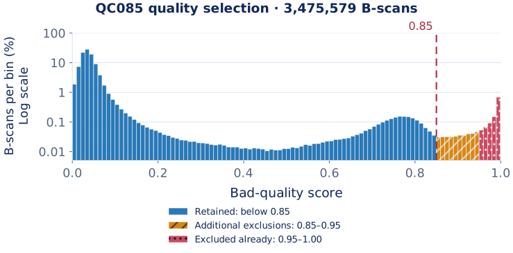
Publishing the histogram makes the selection decision visible: most scores lie near zero, with a smaller high-score tail. The score is an uncalibrated ranking; 0.85 is a cutoff, not an 85% probability of poor quality. Its distribution also gives me a starting point for investigating whether exclusions cluster by acquisition condition.

Measure the same representation on the same images

The monitor periodically evaluates 256 fixed B-scans from the pretraining population. It reduces each full raster by three, applies no augmentation, and averages patch-token features after the encoder’s final LayerNorm. The result is one 1,024-dimensional vector per image, before the projector or decoder.

I center these vectors across images without L2-normalizing each vector. The squared singular values of this centered matrix describe how its variation is distributed. Writing those values as λ, the two plotted summaries are:

PC1 share = largest λ / sum(λ) Participation ratio = sum(λ)² / sum(λ²)

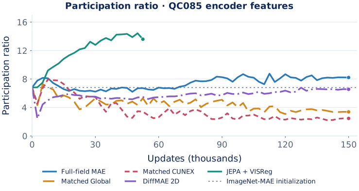
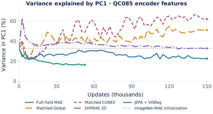
PC1 share measures how much variation lies in the strongest direction. Participation ratio, or PR, measures the effective number of contributing directions. For variances [1, 1, 1, 1], PC1 is 25% and PR is four. For [7, 1, 1, 1], PC1 rises to 70% and PR falls to about 1.92: four directions still vary, but one dominates.

This is why I track both. They reveal concentration that a scalar training loss can hide. The fixed panel removes changes in sampled images from the comparison, while the shared feature extraction makes the measurement consistent across objectives. With 256 centered observations, the measured rank is at most 255, regardless of the encoder’s 1,024 output coordinates.

The recipes produce different feature spectra

All encoders start from the same ImageNet-pretrained MAE checkpoint. The zero-update reference therefore measures the representation before domain pretraining.

Participation ratio starts near 6.8. JEPA reaches 13.59 at update 52,500. At update 150,000, full-field MAE is 8.21, DiffMAE 6.56, Matched Global 3.38, and Matched CUNEX 2.47. — **Encoder geometry through training**Fixed panel of 256 training-distribution images

Encoder or run	Updates in snapshot	Participation ratio	PC1 share
ImageNet-MAE initialization	0 domain updates	6.81	32.7%
Full-field MAE	150,000	8.21	22.5%
Matched-Global	150,000	3.38	50.9%
Matched-CUNEX	150,000	2.47	61.8%
DiffMAE 2D	150,000	6.56	32.7%
JEPA + VISReg	52,500	13.59	16.3%

The clearest contrast is between full-field reconstruction and the matched-patch arms. Full-field MAE increases PR from 6.81 to 8.21 and reduces the leading direction’s share. Both matched arms move toward greater concentration; in Matched-CUNEX, one direction accounts for nearly 62% of the measured variation.

DiffMAE ends close to the initialization on these two summaries. JEPA reaches PR 13.59 and PC1 16.3%, the broadest spectrum among the displayed checkpoints. Its curve stops at the recorded 52,500-update diagnostic; the other four arms have completed 150,000 updates. The table compares those checkpoint positions, rather than equal training endpoints.

Each update presents 64 source images. The full 150,000-update budget is therefore 9.6 million presentations, approximately 2.8 passes over the retained corpus. JEPA’s ten views increase its computation per source; they do not multiply the number of source-image passes.

What I learned from the concentration

The matched arms make spatial sampling a concrete research question. They share a limited patch budget but place patches differently: Matched-Global samples the grid, while Matched-CUNEX uses a segmentation mask. Both concentrate relative to their initialization. That makes restricted context a plausible explanation to test, alongside masking and optimization; these curves alone do not isolate the cause.

JEPA’s result has a different interpretation because its VISReg regularizer explicitly shapes representation geometry. Although the monitor reads encoder features before the projector, the regularizer’s gradients train the encoder too. The observed dispersion is consistent with that objective.

The boundary for all these findings is the same: PR and PC1 measure feature geometry on an in-sample panel, not diagnostic performance. Directions may encode anatomy, acquisition conditions, or both; similar spectra can also represent different distinctions. I use the measurements to identify behavior worth testing in a patient-separated downstream comparison, without turning them into an encoder leaderboard.

Make the global–local recipe practical

JEPA combines two full-field views with eight native local views. Running that workload on two NVIDIA L40S GPUs required preserving the full-batch objective while distributing encoder work. I kept the batch of 64 sources, the 640-representation projector population, the global objective and gradient clipping, and BF16 precision unchanged.

The performance investigation found a useful distinction between where a wait appears and what causes it. A trace showed rank zero spending about 1.48 seconds in all-gather, the operation that collects work from both GPUs. The other rank was late because its CPU input and view preparation had not finished. Making communication faster would not remove that upstream delay.

I changed the coordinator to prepare the next native batch and its first views while the GPUs computed the current update. This preserved source order and random-number state while overlapping preparation with useful GPU work.

The matched, unprofiled ABBA comparison ran the original and optimized variants in A–B–B–A order on the same workload, retaining ten update measurements per variant:

Measurement	Original	With input prefetch
Mean time per optimizer update	10.246 s	8.787 s
Observed range	10.024–10.511 s	8.618–8.935 s

That is 14.2% less time per update, or a 1.166× speedup. The timing includes input waiting, forward and backward computation, validity checks, gradient clipping, and AdamW. Periodic diagnostics and checkpoint saves are outside this timing window. After resuming the training run, a separate 20-update window averaged 8.799 seconds.

Correctness was part of the change: inputs, features and loss scalars matched exactly, as did 303 gradient tensors and 1,221 model/optimizer-state tensors. The two ranks agreed, and the resume comparison was bit-identical. These checks let me deploy the optimization without changing the experiment to obtain the speedup.

The compute-bound finding comes from profiling

In a 26 September Nsight Compute capture, I inspected eight BF16 matrix-multiplication launches from a checkpoint replay. Measured compute throughput was 78.66–89.70% of the relevant peak, compared with 54.83–61.31% memory throughput. ML Training Monitor classified all eight sampled kernels as primarily compute-limited.

The 30 September optimized two-GPU trace then showed where the full update spent its time. GPU kernels occupied about 90% of each rank’s measured step, including about 7.9 seconds per GPU outside the NCCL communication library. Rank zero’s all-gather duration was about 36 milliseconds. Both GPUs were simultaneously idle for only 146 milliseconds of the 8.893-second aligned capture.

Together, the kernel counters and execution timeline support a GPU-compute-dominated optimized step. No other large isolated avoidable delay was identified in that trace. The trace explains execution; the separate unprofiled comparison establishes the measured speedup.

The next research question

These experiments have established different representation trajectories and a faster, equivalent way to run the global–local recipe. The next question is which distinctions the encoders make accessible for a defined clinical task.

The prepared downstream pools contain 562 development patients with 23,891 B-scans and 140 reserved patients with 6,142 B-scans. Task-specific eligibility and labels will determine the final denominators. A common patient-separated protocol can compare frozen-encoder probes and fine-tuning, with checkpoint selection performed on development data. That connects the geometry observed here to measurable task performance.

Data and measurement record

The aggregate snapshot and definitions contain the histogram counts, spectral curves, checkpoint positions and measurement scopes used in these figures. They were saved on 30 September 2026 at 22:15:56 UTC and remain a dated record as training continues.

The profiling summary records the separately dated Nsight kernel capture and two-GPU qualification. Hardware-counter definitions are documented in the Nsight Compute profiling guide.

The workflow is available as ML Training Monitor. Its separate 48-second demonstration uses labeled synthetic telemetry. The research figures and performance measurements in this article come from the recorded experiments.