What Are Zernike Polynomials?

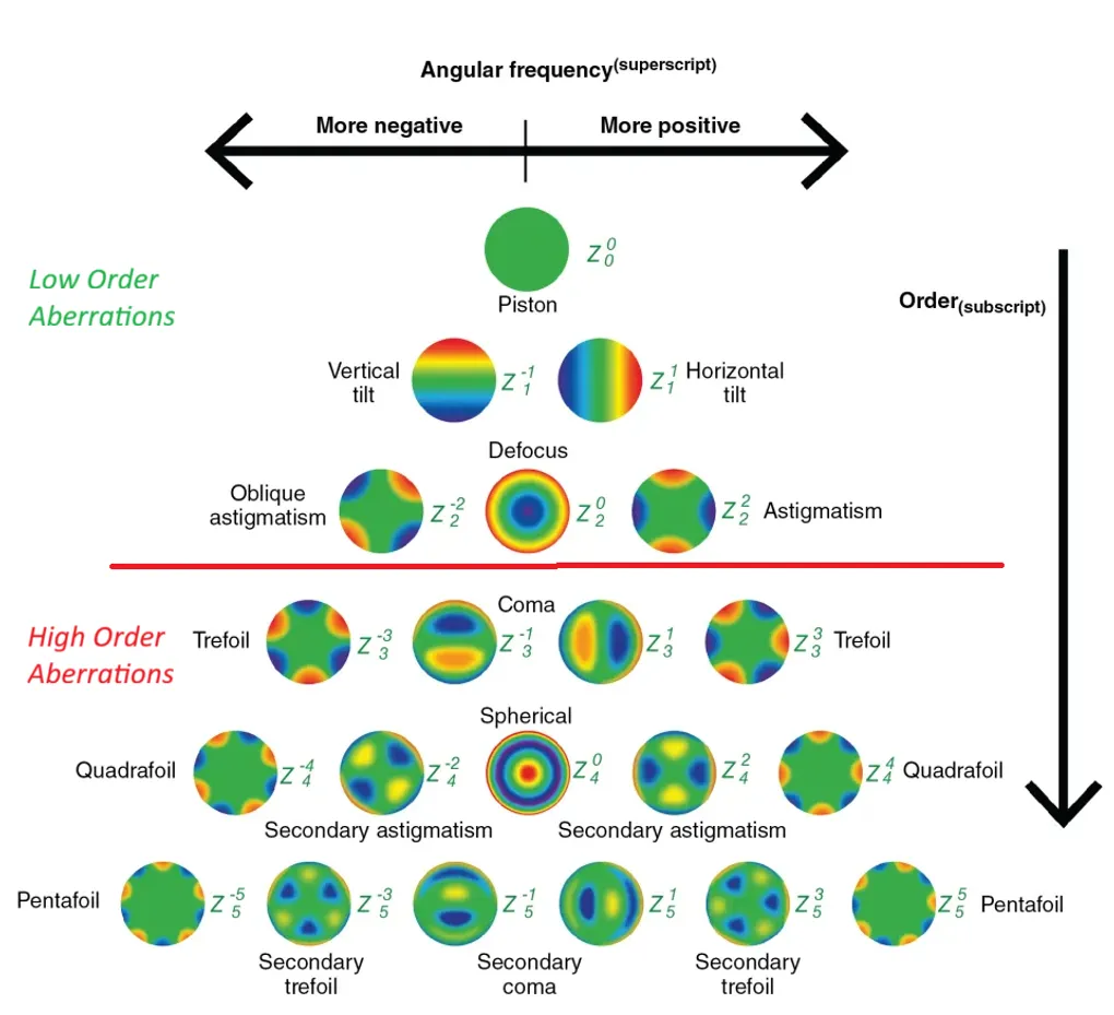
Zernike polynomials are a set of orthogonal functions defined over the unit disk in polar coordinates (ρ, θ). Each polynomial is indexed by a radial degree n and azimuthal frequency m, producing patterns with familiar names: piston, tilt, defocus, astigmatism, coma, trefoil, spherical aberration, and so on through higher orders. Their orthogonality means you can decompose any smooth function on a circular aperture into these modes without redundancy — which is exactly why they became the standard representation for optical wavefronts.

In ophthalmology, they describe how light bends as it passes through the cornea and lens. The decomposition breaks aberrations into distinct, interpretable components, and that turns out to be the right abstraction for both clinical diagnosis and machine learning.

Low-Order vs. High-Order Aberrations

Aberrations split into two broad categories. Low-order aberrations (LOAs) — myopia, hyperopia, astigmatism — are the familiar ones. They stem from the overall shape of the eye and are correctable with glasses, contacts, or standard refractive surgery.

High-order aberrations (HOAs) are different. Coma, trefoil, spherical aberration — these arise from subtle irregularities in the corneal surface, whether from scars, trauma, or disease. Glasses can’t correct them. Patients with significant HOAs experience glare, halos around lights, reduced contrast sensitivity, and degraded night vision that conventional optics won’t fix.

Why This Matters: Keratoconus

In keratoconus, the cornea thins and bulges into a cone, which amplifies HOAs dramatically. Light rays hit the retina at inconsistent angles instead of converging cleanly. The result: blurred, distorted vision that worsens over time. Halos around lights, severe glare, poor night vision, difficulty reading or recognizing faces. Driving at night becomes dangerous, screen work causes fatigue. It’s a condition that quietly erodes quality of life in ways that are hard to appreciate until you see the comparison above.

From Raw MS-39 Data to Zernike Coefficients

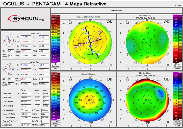
The MS-39 (CSO) combines Placido-disk topography with spectral-domain OCT to capture detailed maps of the cornea’s anterior and posterior surfaces — pachymetry, elevation, curvature, dioptric power — across multiple diameter zones. The raw output is a set of CSV files with polar-coordinate measurements.

The problem: these raw measurements aren’t directly useful for ML. They’re noisy, device-specific, and high-dimensional in unhelpful ways. Zernike decomposition compresses them into a compact, physically meaningful feature set where each coefficient maps to a specific type of optical aberration with a known clinical interpretation.

My pipeline transforms the raw MS-39 exports into ML-ready Zernike coefficients through five stages:

1. Data ingestion — parse CSV exports across 2–7mm diameter zones for anterior, posterior, and stromal surfaces
2. Best-fit sphere centering — fit a reference sphere to isolate clinically relevant aberrations from baseline curvature
3. Zernike fitting — least-squares decomposition up to order 6
4. OPD correction — convert geometric coefficients to optical path difference units, following the clinical convention of centering on the corneal apex
5. Output — structured CSVs and visualization maps for validation

Pipeline Implementation

1. Data Ingestion and Preprocessing

Extracts elevation data from MS-39 CSV files across multiple diameter zones, filtering out noise and invalid values. The parser is tailored for the MS-39’s polar-coordinate export format.

def process_single_csv_zones(p):
    r = {'filename': os.path.basename(p), 'surfaces': {}}
    for sn, sr, nr, mn, mx in segments:
        ss, m = sn.replace('elevation_', ''), lire_segment(p, sr, nr)
        if m.empty: continue
        m = m.mask((m < mn) | (m > mx)).replace(-1000, np.nan)
        r['surfaces'][ss] = {}
        for dia in [2, 3, 4, 5, 6, 7]:
            zd = extract_diameter_zones(m, dia)
            if zd is not None: r['surfaces'][ss][f'{dia}mm'] = {'data': zd}
    return r

2. Best-Fit Sphere Centering

Fits a sphere to the elevation data via least-squares optimization, then computes residual maps relative to that sphere. This step is critical — without it, you’d only see standard refractive aberrations. Subtracting the best-fit sphere isolates the irregular component, which is what matters for clinical diagnosis and downstream ML.

def calculate_bfs(zd,rs=0.2):
    x,y,z=polar_to_cartesian_coords(zd,rs)
    if len(x)<4:return None,None
    zr=np.max(z)-np.min(z)
    er=np.clip((np.max(np.sqrt(x**2+y**2))**2)/(2*zr),6.,15.) if zr>1e-3 else 8.
    ig=[0.,0.,np.max(z)+er,er]
    res=least_squares(bfs_residuals,ig,args=(x,y,z),method='lm',max_nfev=1000)
    if not res.success or not (abs(res.x[0])<5 and abs(res.x[1])<5 and 4.<res.x[3]<20.):return None,None
    return {'center_x':res.x[0],'center_y':res.x[1],'center_z':res.x[2],'radius':res.x[3],'rms_residual':np.sqrt(np.mean(res.fun**2)) },{'n_points':len(x),'convergence':res.success}

3. Zernike Coefficient Fitting

Fits Zernike polynomials up to order 6 to the residual maps via least-squares. Each coefficient quantifies a specific aberration mode, producing a compact feature vector that’s both interpretable and ML-ready.

def fit_zernike_coefficients(x,y,z,mo,pr):
    vm=np.isfinite(x)&np.isfinite(y)&np.isfinite(z)
    xv,yv,zv=x[vm],y[vm],z[vm]
    if len(xv)<10:return None,None,None
    rho,theta=np.sqrt(xv**2+yv**2)/pr,np.arctan2(yv,xv)
    i=rho<=1.001
    rho,theta,zv=rho[i],theta[i],zv[i]
    if len(rho)<10:return None,None,None
    modes=generate_zernike_modes(mo)
    A=np.vstack([zernike_polynomial(n,m,rho,theta) for j,n,m,name in modes]).T
    c,_,_,_=np.linalg.lstsq(A,zv,rcond=None)
    if not np.all(np.isfinite(c)):return None,None,None
    zf=A@c
    ve=100*(1-np.sum((zv-zf)**2)/np.sum((zv-np.mean(zv))**2)) if np.var(zv)>1e-12 else 100.
    return c,modes,{'rms_residual':np.sqrt(np.mean((zv-zf)**2)),'n_points_fitted':len(rho),'variance_explained_pct':ve}

4. OPD Correction

Converts geometric coefficients to optical path difference (OPD) units and zeros the piston term. This follows the clinical convention where the origin sits at the corneal apex rather than the geometric center — a subtle but important distinction when matching industry-standard measurements from devices like the MS-39.

def apply_opd_and_convention_correction(coefficients_mm, modes):
    correction_factor = -0.376
    corrected_coefficients_mm = np.array(coefficients_mm) * correction_factor
    if len(corrected_coefficients_mm) > 0:
        corrected_coefficients_mm[0] = 0.0
    return corrected_coefficients_mm

5. Visualization and Output

Exports Zernike coefficients to structured CSVs — both geometric and OPD-corrected — and generates aberration maps for visual validation. In healthcare ML, being able to inspect and trust intermediate outputs isn’t optional.

def save_results_to_csv(ar, of):
    sf = {k: v for k, v in ar['files'].items() if v.get('status') == 'success'}
    if not sf: return
    all_geom_results, all_opd_results = [], []
    rm = generate_zernike_modes()
    ts = datetime.now().strftime("%Y-%m-%d_%H-%M-%S")
    for fn, fd in sf.items():
        geom_file_row = {'filename': fn}
        opd_file_row = {'filename': fn}
        for sn, sd in fd.get('zernike_results', {}).get('surfaces', {}).items():
            for zn, zd in sd.items():
                p = f"{sn}_{zn}"
                c_geom = zd.get('coefficients_geometric_mm')
                c_opd = zd.get('coefficients_opd_corrected_mm')
                for j, n, m, name in rm:
                    geom_file_row[f'{p}_zernike_z{j}_{name}_um'] = c_geom[j] * 1000 if c_geom is not None and j < len(c_geom) else np.nan
                    opd_file_row[f'{p}_zernike_z{j}_{name}_um'] = c_opd[j] * 1000 if c_opd is not None and j < len(c_opd) else np.nan
        all_geom_results.append(geom_file_row)
        all_opd_results.append(opd_file_row)
    df_geom = pd.DataFrame(all_geom_results)
    df_opd = pd.DataFrame(all_opd_results)
    df_geom.to_csv(os.path.join(of, f"batch_results_geom_{ts}.csv"), index=False, sep=';', float_format='%.6f')
    df_opd.to_csv(os.path.join(of, f"batch_results_opd_{ts}.csv"), index=False, sep=';', float_format='%.6f')

What This Enables

The Zernike coefficients produced by this pipeline are the feature engineering foundation for the ML work described in my other post on predicting surgical outcomes. Each coefficient maps to a clinically interpretable aberration — coma, spherical aberration, trefoil — so the ML models operate on features that ophthalmologists already understand and trust. That interpretability matters when your model’s predictions feed into surgical decisions.